This session borrows from the open-source lecture materials by Jeremy Orloff and Jonathan Bloom, MIT, Central Limit Theorem and the Law of Large Numbers, and from the lecture slides in the courses Quantitative Methods I and III (Georgetown University, PhD in Government).
Law of Large Numbers:
Suppose that each random variable \(X_i\) is an independent flip of a coin, where each head flip is coded as 1 and each tail flip as 0. \(\overline{X}_n\) would be the “headcount” of n flips. We expect the share of heads to be half. This is not guaranteed however, due to the element of random error.
In simple terms, the Law of Large Numbers states that the more often we flip the coin, the more the shares of heads and tails will balance out. In other words, for larger n, the mean of \(\overline{X}_n\) will approach 0.5.
One way of testing this is to consider the coin flip as a random variable drawn from the Bernoulli Distribution: \(X_i \sim Bernoulli(0.5)\) and \(\mu = 0.5\). The Bernoulli Distribution describes a special case of the Binomial Distribution where only one trial is conducted, whose probability of success (no matter how defined) is \(p\) and failure \(q = 1-p\).
What we’re looking to see is the clustering of the average around 0.5. To do that, we will look at the probability of getting a sample average within a tenth of 0.5 (a share of heads in a sample of coin flips between 40 and 60 percent). We expect the probability of landing in that range to increase the more flips we conduct:
This law reveals that the more samples we take, the likelihood of getting a sample mean \(\overline{X}_n\) within an infinitesimally small radius around the true population mean \(\mu\) becomes almost certain. We call this convergence in probability, because the sample mean (\(\overline{X}_n\)) may not indeed converge in value, that is becomes identical to the true population mean (\(\mu\)). Yet, the likelihood of obtaining a value close to the true mean becomes almost certain (How close? As small as you’d like the difference, \(\epsilon\) to be).
Convergence in Probability is the notion that underlies consistency in estimators. We say that an estimator is consistent when it converges in probability to the true parameter, the more samples we get.
Another mathematical formulation of this intuition is embodied in the Strong Law of Large Numbers which states that the more samples we draw, then the probability of the average sample mean equating the true population mean becomes almost certain.
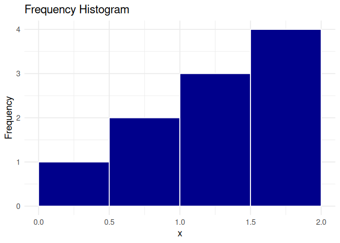
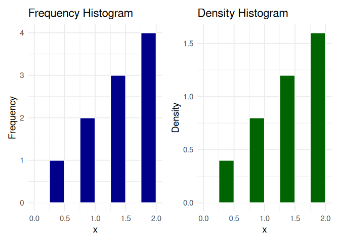
# Frequency histogramp1 <-ggplot(df, aes(x = x)) +geom_histogram(breaks =seq(0, 2, by =0.5),fill ="darkblue", color ="white" ) +labs(title ="Frequency Histogram",x ="x", y ="Frequency" ) +theme_minimal(base_size =14)p1
Code
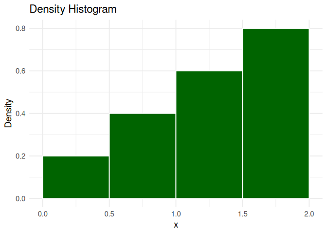
# Density histogramp2 <-ggplot(df, aes(x = x)) +geom_histogram(aes(y =after_stat(density)), breaks =seq(0, 2, by =0.5),fill ="darkgreen", color ="white" ) +labs(title ="Density Histogram",x ="x", y ="Density" ) +theme_minimal(base_size =14)p2
Code
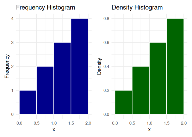
p1 + p2
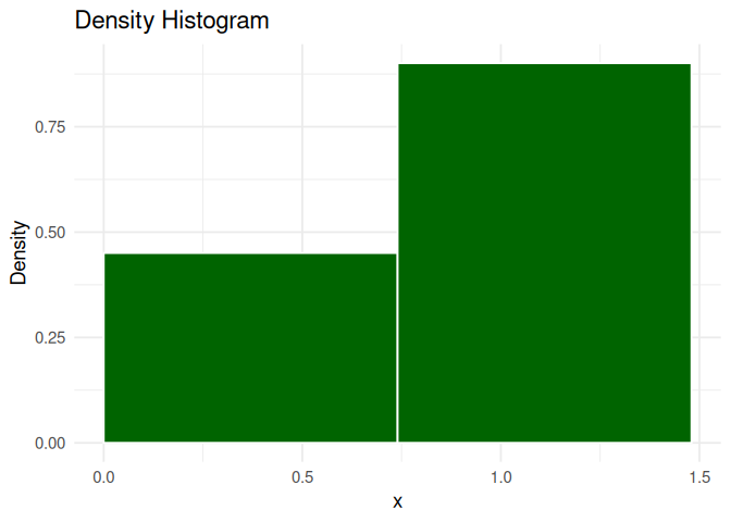
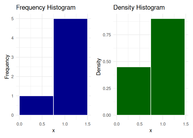
The height of the bar in a frequency histogram gives the number of data points that fall within that interval, while the height of the bar in the density histogram shows the relative likelihood of observing data points per unit of X. Multiplying this density with the bin-width gives us the share or proportion of observations that fall within that interval.
Note that values on the bin boundaries are put into the left-hand bin. We call these bins are right-closed (for values in a right-closed interval).
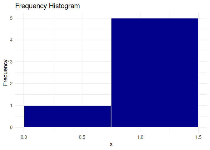
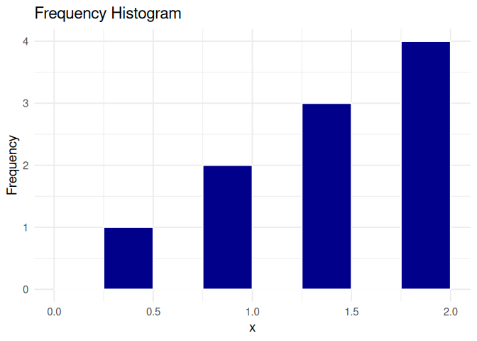
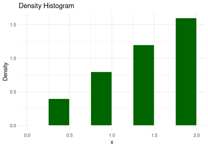
The shape of any histogram depends on the chosen band-width!
# Using wide bin-widthsx <-c(0.5, 1, 1, 1.5, 1.5, 1.5, 2, 2, 2, 2)df <-data.frame(x)# Frequency histogramp1 <-ggplot(df, aes(x = x)) +geom_histogram(breaks =seq(0, 2, by =0.75),fill ="darkblue", color ="white" ) +labs(title ="Frequency Histogram",x ="x", y ="Frequency" ) +theme_minimal(base_size =14)p1
# Density histogramp2 <-ggplot(df, aes(x = x)) +geom_histogram(aes(y =after_stat(density)), breaks =seq(0, 2, by =0.74),fill ="darkgreen", color ="white" ) +labs(title ="Density Histogram",x ="x", y ="Density" ) +theme_minimal(base_size =14)p2
p1 + p2
# Using narrow bin-widths# Frequency histogramp1 <-ggplot(df, aes(x = x)) +geom_histogram(breaks =seq(0, 2, by =0.25),fill ="darkblue", color ="white" ) +labs(title ="Frequency Histogram",x ="x", y ="Frequency" ) +theme_minimal(base_size =14)p1
# Density histogramp2 <-ggplot(df, aes(x = x)) +geom_histogram(aes(y =after_stat(density)), breaks =seq(0, 2, by =0.25),fill ="darkgreen", color ="white" ) +labs(title ="Density Histogram",x ="x", y ="Density" ) +theme_minimal(base_size =14)p2
p1 + p2
From density histograms to PDFs:
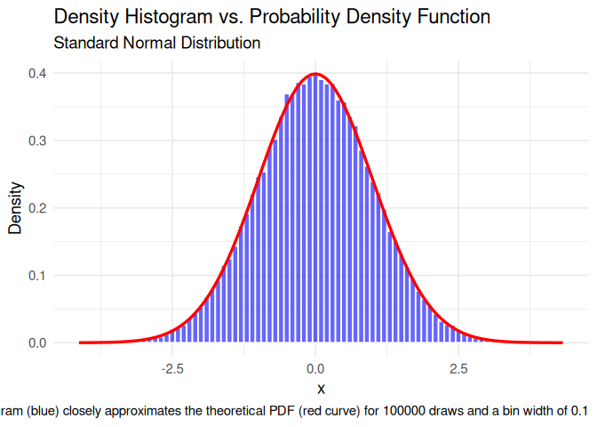
The Probability Density Function of a given distribution is the continuous analog of the density histogram. One could also say that the density histogram is an empirical estimate or snap shot of the PDF. The density histogram is drawn using finite data. The Probability Density Function shows the overall density under ever more observations and a diminishing bin-width, i.e., it is a smooth, theoretical limit of the histogram.
In other words:
\[ PDF(x) = lim_{\, bins \rightarrow 0\, , \, \, n \rightarrow \infty} \, \text{height of density histogram at x}\]
Similarly, calculating the likelihood of observing data points within a given interval changes from multiplying the height and the width of the interval bar to calculating the area under the curve:
\[ P(a \le X \le b) = \int_{a}^{b} f(x) \, dx\]
Code
# Generate 100000 random draws from the standard normal distributionset.seed(123) x <-rnorm(100000)df <-data.frame(x = x)ggplot(df, aes(x = x)) +geom_histogram(aes(y =after_stat(density)), # scale to density (area = 1)binwidth =0.1, # bin width of 0.1fill ="blue", color ="white",alpha =0.6 ) +stat_function(fun = dnorm, # standard normal PDFargs =list(mean =0, sd =1),color ="red",linewidth =1.2 ) +labs(title ="Density Histogram vs. Probability Density Function",subtitle ="Standard Normal Distribution",caption ="Histogram (blue) closely approximates the theoretical PDF (red curve) for 100000 draws and a bin width of 0.1",x ="x",y ="Density" ) +theme_minimal(base_size =14)
Central Limit Theorem:
The CLT states that the relative proportions of different outcomes from a group of random variables (independent and identically distributed) will be approximately normal. This holds no matter the initial underlying distribution of the random variables.
The mathematical formulation is the following:
Let \(X_1, X_2, ..., X_n\) be i.i.d. random variables each having mean \(\mu\) and standard deviation \(\sigma\). For each n, let \(S_n\) denote the sum and let \(\overline{X}_n\) be the average:
\(\overline{X}_n\) is often denoted the sample mean. Any sample mean we compute is but one realization of this random variable
In other words:
The sample mean (average of random variables) \(\overline{X}_n\) approximates a normal distribution with the same mean as all of the underlying random variables but a smaller standard deviation (\(\sigma/\sqrt(n)\)).
The sum of the random variables approximates a normal distribution.
Standardized, either approximates a standard normal distribution.
Why do we care about the CLT? and the normal distribution? and what role do they serve in hypothesis testing?
The Central Limit Theorem allows us to approximate a normal distribution, even when the underlying population (our point of origin) is not normally distributed. It demonstrates the idea that randomness in any given random variable tends to diminish when aggregated with other identically drawn, and independent random variables. It allows us to make precise statements about the distribution of outcomes over a large number of events, even if each single manifestation is random and chaotic.Now the normal distribution has probability features which are extremely useful for computations.
Why is this relevant in the regression setup?
Assume a standard linear regression model:
\[ Y = X \beta + \epsilon\]
Then OLS BLUE Estimator is:
\[ \hat\beta = (X'X)^{-1} X' Y \]
which is equal to:
\[ \hat\beta = \beta + (X'X)^{-1} X' \epsilon \]
We can view our estimator as a weighted sum of random errors, i.e., a linear combination of many independent random variables (assuming the errors are i.i.d.). The CLT applies to linear combinations of random variables. Each estimated coefficient measures an average marginal effect, holding all else constant. The estimate is a sample statistic, computed based on many noisy data points with their own (independent) small disturbances. The “marginal effect” in a regression is one realization of a broader sampling distribution that behaves like a sample mean. That’s why we can use t-statistics, confidence intervals, and p-values based on normal approximations.
Recall that the sample mean we compute is but one realization of the random variable (\(\overline{X}_n\)). We simply assume that, had we observed many instances of this random variable, they would take a normal shape. Hence, we treat the observed sample mean as belonging to a broader, normally distributed, family. Having that in mind, we ascertain the statistical significance of an estimated parameter, when observing it is “unlikely enough” given a normal distribution centered at mean 0 (null hypothesis).